Standard Atmosphere
Contents
Standard Atmosphere#
Aerodynamic analyses need various air properties to do the calculations. The standard way to come up with thoseproperties is to use the Standard Atmosphere model, published in 1976. There is a Python package that provides access to this model, but for our purposes, I will use methods defined in Mark Drela’s Flight Vehicle Aerodynamics[Dre14].
To get started with this model, we need to define the properties at sea-level. Each of these properties has engineering units attached to the number. It is critical that these units be consistent in calculations, so we will use the Python pint package to add these units to the data.
import pint
u = pint.UnitRegistry()
rho_SL = 1.225*u.kg/u.m**3
rho_SL
p_SL = 1.0132e5*u.pascal
p_SL
T_SL = 288.15*u.kelvin
T_SL
a_SL = 340.3*u.m/u.sec
a_SL
mu_SL = 1.79e-5*u.kg/(u.m*u.sec)
mu_SL
The equations that define these properties for altitudes other than sea-level are given in Drela’s book, but they originally come from the COESA Working Group[Gro76]
\begin{equation} p(z) = e^{-0.118z -\frac{0.0015z^2}{1-0.018z+0.0011z^2}} \end{equation}
import matplotlib.pyplot as plt
import numpy as np
alt = np.linspace(0,26,27)*u.km
alt
| Magnitude | [0.0 1.0 2.0 3.0 4.0 5.0 6.0 7.0 8.0 9.0 10.0 11.0 12.0 13.0 14.0 15.0 |
|---|---|
| Units | kilometer |
Pressure vs Altitude#
def p(z):
    zm = z.magnitude
    return p_SL*np.exp(-0.118*zm-(0.0015*zm**2)/(1-0.018*zm+0.0011*zm**2))
poa = p(alt)
poa
| Magnitude | [101320.0 89905.40296142412 79526.3201763238 70116.7008535207 |
|---|---|
| Units | pascal |
popsl = poa/p_SL
Temperature vs Altitude#
def T(z):
    zm = z.magnitude
    res = 216.65 + 2.0*np.log(1 + np.exp(35.75 - 3.25*zm) + np.exp(-3.0+0.0003*zm**3))
    return res*u.kelvin
T(0*u.km)
totsl = T(alt)
totsl = totsl/T_SL
totsl
| Magnitude | [1.0 0.9774423043553707 0.9548846087107425 0.9323269130661487 |
|---|---|
| Units | dimensionless |
Viscosity vs Altitude#
The viscosity function is given next:
\begin{equation} \mu(z) = \mu(T(z)) = \mu_{SL}\left(\frac{T}{T_{SL}} \right)^\frac{3}{2}\frac{T_{SL} + T_S}{T + T_S} \end{equation}
From Sutherland’s Law, the value for \(T_S\) is \(110K\) for air.
T_S = 110 * u.kelvin
temp = T(alt)
temp
| Magnitude | [288.15 281.65000000000003 275.15000000000043 268.6500000000107 |
|---|---|
| Units | kelvin |
def mu(z):
    temp = T(z)
    return mu_SL*(temp/T_SL)**1.5*(T_SL + T_S)/(temp+T_S)
muoa = mu(alt)
muoa
| Magnitude | [1.79e-05 1.7584835809587085e-05 1.7266177001104793e-05 |
|---|---|
| Units | kilogram/(meter second) |
Density vs Altitude#
To get density we need to use the ideal gas state equation
\begin{equation} p = \rho R T \end{equation}
Where the gas constant is \(R = 287.04\frac{J}{kgK}\)
Rgas = 287.04*u.joule/(u.kg*u.kelvin)
def rho(z):
    temp = T(z)
    press = p(z)
    rho = press/(Rgas*temp)
    return rho
rho(alt).to_base_units()
| Magnitude | [1.2249944916355073 1.1120738151154193 1.006929231672808 |
|---|---|
| Units | kilogram/meter3 |
rhooa = rho(alt)
rhooa = rhooa/rho_SL
Speed of Sound vs Altitude#
The speed of sound is calculated using this formula:
\begin{equation} a= \sqrt{\gamma RT} \end{equation}
gamma = 1.4
def sos(z):
    temp = T(z)
    res = np.sqrt(gamma*Rgas*temp)
    return res
sosoa = sos(alt).to_base_units()
aoasl = sosoa/a_SL
plt.plot(popsl,alt)
plt.ylabel("z(km)")
plt.plot(totsl, alt, label=r"$p/p_{sl}$")
plt.plot(muoa/mu_SL,alt, label=r"$\mu/\mu_{sl}$")
plt.plot(rhooa,alt, label = r"$\rho/\rho_{sl}$")
plt.plot(aoasl,alt, label = r"$a/a_{sl}$")
plt.legend()
/Users/rblack/_dev/mmqprop/.venv/lib/python3.10/site-packages/matplotlib/cbook/__init__.py:1369: UnitStrippedWarning: The unit of the quantity is stripped when downcasting to ndarray.
  return np.asarray(x, float)
<matplotlib.legend.Legend at 0x10dacafe0>
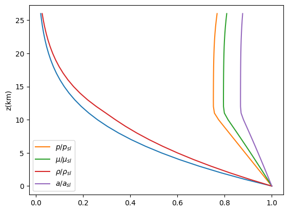
That plot looks like the figure presented in Drela’s book.
All of this code has been placed in a single class names StdATm which takes an altitude in meters, and returns the properties as a dictionary. We can nhand this function a ((numpy** array of altitudes is needed.))
import sys
import os
sys.path.insert(0, '../../..')
from mmqprop.StdAtm import StdAtm
s = StdAtm(u,alt)
s.properties().to_base_units()
| Magnitude | [340.28635940924806 336.4264294017341 332.52169613425247 328.5705622845788 |
|---|---|
| Units | meter/second |
..literalinclude:: ../../mmqprop/StdAtm.py