Experiments with Burger’s Equation

The original code developed for this study was written in Fortran IV, and used global variables for everything! I rewrote that program in Python* in 2003 as part of a course in Object Oriented Design, but did not tap into the real power of modern Python libraries. My goal is to fix that problem.

Burger’s Equation

The first example we will consider is Burger’s Equation. I am borrowing code from Lorena Barba’s CFD Python: the 12 steps to Navier-Stokes equations [BF19]. Here is the basic equation.

(1)\[\begin{equation} \frac{\partial u}{\partial t} + u \frac{\partial u}{\partial x} = \nu\frac{\partial^2 u}{\partial x^2} \end{equation}\]

### Initial Conditions

There is an analytic solution available for this equation, useful for checking errors:

If we use these initial conditions:

(2)\[\begin{equation} u = - \frac{2\nu}{\phi}\frac{\partial \phi}{\partial x} + 4 \end{equation}\]

(3)\[\begin{equation} \phi = exp \Bigl(\frac{-(x - 4t)^2}{4\nu(t + 1} \Bigr) + exp\Bigl( \frac{-(x - 2\pi)^2}{4\nu}\Bigr) \end{equation}\]

Then, the analytic solution is given as:

(4)\[\begin{eqnarray} u &= -\frac{2 \nu}{\phi} \frac{\partial \phi}{\partial x} + 4 \\ \phi &= \exp \bigg(\frac{-(x-4t)^2}{4 \nu (t+1)} \bigg) + \exp \bigg(\frac{-(x-4t -2 \pi)^2}{4 \nu(t+1)} \bigg) \end{eqnarray}\]

The boundary condition is:

\[u(0) = u(2\pi)\]

A simple finite difference representation of this equation looks like this:

\[\frac{u_i^{n+1}-u_i^n}{\Delta t} + u_i^n \frac{u_i^n - u_{i-1}}{\Delta x} = \nu \frac{u_{i+1} - 2u_i + u_{i-1}}{\Delta x^2}\]

Given an initial condition, the only unknown is \(u_i^{n+1}\). We can “march” this code in time to see how the solution evolves.

\[u_i^{n+1} = u_i - u_i \frac{\Delta t}{\Delta x} (u_i - u_{i-1}) + \nu \frac{\Delta t}{\Delta x^2}(u_{i+1} - 2u_i + u_{i-1})\]

The code provided in the 12-Step lecture runs the iteration through all timesteps and displays the final solution. I think it would be more interesting to watch the solution evolve. Since we showed code that animates the PNS solver solution, all we need to do is adapt that here.

SInce this problem is so simple, I will simply let the animation code step the solution. Each time the animation code calls fetch data, we run the solver code and return the results.

First set up access to the required libraries: np for data, and matplotlib for graphics.

import numpy as np
import matplotlib.pyplot as plt
%matplotlib inline

Next we set up parameters for the solution run

nx = 41
sigma = 0.5
dx = 2./(nx-1)
nt = 20    #the number of timesteps we want to calculate
nu = 0.3   #the value of viscosity
dt = sigma*dx**2/nu #dt is defined using sigma ... more later!

sigma is a parameter that controls the stability of this solution scheme. The original code used a value os 0.2. I have modified this to 0.5 here to show the problem.

Now, we set the initial conditions

u = np.ones(nx)      #a numpy array with nx elements all equal to 1.
u[int(.5/dx) : int(1/dx+1)]=2  #setting u = 2 between 0.5 and 1 as per our I.C.

We will calculate new values and save them in the un array

un = np.ones(nx) #our placeholder array, un, to advance the solution in time

Now for the actual time iteration loop. This one runs nt steps

for n in range(nt):  #iterate through time
    un[:] = u[:] ##copy the existing values of u into un
    for i in range(1,nx-1):
        u[i] = un[i] + nu*dt/dx**2*(un[i+1]-2*un[i]+un[i-1])

Notice that we only perform this loop from the second point to one less than the last point in the u aray. The two end points are left untouched. This establishes the boundary conditions for the solution.

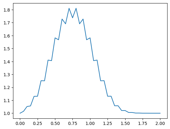
when this code completes, we can display the final solution (well, the solution after the number of time steps we chose).

plt.plot(np.linspace(0,2,nx), u)

[<matplotlib.lines.Line2D at 0x10fdd5810>]

from matplotlib import animation, rc
from IPython.display import HTML

import sys
sys.path.insert(1, '/Users/rblack/_dev/CFD-talk/Python')

# First set up the figure, the axis, and the plot element we want to animate
fig, ax = plt.subplots()

# the test animation will display the selected property 
# curves Values run from 
ax.set_xlim((0.0, 2.0))
ax.set_ylim((1.0, 2.0))
plt.title("Burger's Equation")
plt.xlabel("X")
plt.ylabel("U")
plt.grid(color = 'green', linestyle = '--', linewidth = 0.5)
line, = ax.plot([], [], lw=2)

# reset the initial condition
u = np.ones(nx)
xl = int(0.5/dx)
xh = int(1/dx+1)
u[int(.5/dx) : int(1/dx+1)]=2
(xl,xh)

(10, 21)

def init():
    line.set_data([], [])    
    return (line,)

def fetchDataLine(u,i):
    '''generate data line for next time step'''
    un[:] = u[:] ##copy the existing values of u into un
    for i in range(1,nx-1):
        u[i] = un[i] + nu*dt/dx**2*(un[i+1]-2*un[i]+un[i-1])
    return u

# animation function. This is called sequentially
def animate(i):
    x = np.linspace(0, 2, nx)
    y = fetchDataLine(u,i)
    line.set_data(x, y)
    return (line,)
    

anim = animation.FuncAnimation(fig, animate, init_func=init,
                               frames=481, interval=50, blit=True)

HTML(anim.to_html5_video())

At this point, you can play with the value of sigma and see how it affects the solution. Try 1.0, then 0.2 to se the dramatic difference!

A Jupyter NOtebook is a great way to experiment, and get immediate feedback! That is why this environment is so popular in the world of Data Science.